Note
In all 1D tests dependent variables are (J x Q) arrays
J = number of 1D responses
Q = number of nodes to which the 1D responses have been resampled
One- and two-sample tests
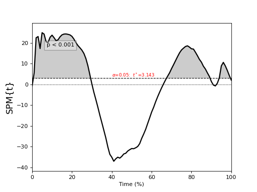
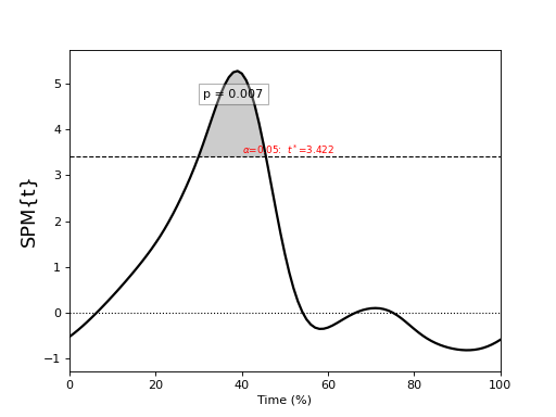
One-sample t test
./spm1d/examples/stats1d/ex_ttest.py
Import necessary packages:
>>> import spm1d
Load a dataset:
>>> dataset    = spm1d.data.uv1d.t1.Random()
>>> Y,mu       = dataset.get_data()  #Y is (10x100), mu=0
Conduct statistical test:
>>> t  = spm1d.stats.ttest(Y, mu)  #mu is 0 by default
>>> ti = t.inference(alpha=0.05, two_tailed=False, interp=True)
>>> ti.plot()
Inference options:
Note
Inference options:
alpha : Type I error rate (0 < alpha < 1). Usually alpha=0.05.
two_tailed : Whether or not to conduct two-tailed inference (True {default} or False). This is applicable only to one- and two-sample tests.
interp : Interpolate clusters to the critical threshold (True {default} or False).
(Source code, png, hires.png, pdf)
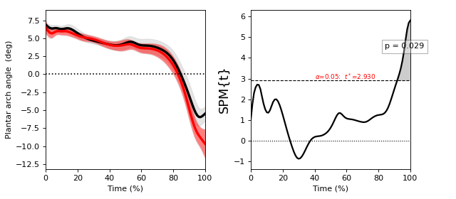
Paired t test
./spm1d/examples/stats1d/ex_ttest_paired.py
Note
A paired t test comparing Y0 to Y1 is equivalent to a one-sample t test of their difference: (Y0 - Y1).
>>> t  = spm1d.stats.ttest_paired(Y0, Y1)
>>> ti = t.inference(alpha=0.05, two_tailed=False)
>>> ti.plot()
(Source code, png, hires.png, pdf)
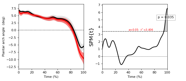
Two-sample t test
./spm1d/examples/stats1d/ex_ttest2.py
Note
- Non-sphericity
spm1d implements a non-sphericity correction when the equal_var keyword argument is set to False.
In general different groups of observations can have different variances, and this should be accounted for unless an assumption of identical variance is justified.
spm1d implements a non-sphericity correction by adjusting the degrees-of-freedom using a the Satterthwaite approximation from restricted maximum likelihood estimates of covariance components.
This non-sphericity correction is available for all tests involving two or more groups.
If you are unsure which is appropriate, set equal_var = False.
>>> t  = spm1d.stats.ttest2(Y0, Y1, equal_var=False)
>>> ti = t.inference(alpha=0.05, two_tailed=False, interp=True)
>>> ti.plot()
ttest2 options:
equal_var : Whether or not to assume equal variance. True or False (default).
(Source code, png, hires.png, pdf)
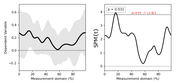
Regression
./spm1d/examples/stats1d/ex_regression.py
Note
If the dependent variable Y is a (J x Q) array, then the independent variable x must be a list or array containing J scalars.
>>> t  = spm1d.stats.regress(Y, x)
>>> ti = t.inference(alpha=0.05)
>>> ti.plot()
These results are from:
Pataky, T. C., Vanrenterghem, J., & Robinson, M. A. (2015). Zero- vs. one-dimensional, parametric vs. non-parametric, and confidence interval vs. hypothesis testing procedures in one-dimensional biomechanical trajectory analysis. Journal of Biomechanics, 1–9. http://doi.org/10.1016/j.jbiomech.2015.02.051
(Source code, png, hires.png, pdf)
General linear model (GLM)
./spm1d/examples/stats1d/ex_glm.py
Danger
Although spm1d.stats.glm permits flexible modeling it does not support non-sphericity corrections. Please use spm1d.stats.glm with caution.
First specify a design matrix X (J x K), where K is the number of modeled factors:
>>> X          = np.zeros((J,nFactors))
>>> X[:,0]     = x       #regresor (continuous variable)
>>> X[:,1]     = 1       #intercept
>>> X[:,2]     = np.linspace(0,1,nCurves)   #linear drift
>>> X[:,3]     = np.sin(np.linspace(0,np.pi,nCurves))  #sinusoidal drift
Then specify a (1 x K) contrast vector:
>>> c = [1, 0, 0, 0] #only the first column is of empirical interest
Then conduct the test:
>>> t  = spm1d.stats.glm(Y, X, c)
>>> ti = t.inference(alpha=0.05)
>>> ti.plot()
(Source code, png, hires.png, pdf)